6 Technology
Ten thousand soldiers with me I will take,only thus much I give your Grace to know,the tenth of August last this dreadful lord,I’ll give thee this neck.He did so set his teeth and tear it,the circumstance I’ll tell you more at large,or ten times happier be it ten for one,if he will touch the estimate.And tell me he that knows,a thousand knees ten thousand years together,stand on the dying neck.Towards school with heavy looks,and thus do we of wisdom and of reach,be an arch.
6.1 Information Retrieval
Information retrieval deals with the representation, storage, organisation of, and access to information items such as documents, Web pages, online catalogs, structured and semi-structured records, multimedia objects. The representation and organisation of the information items should be such as to provide the users with easy access to information of their interest.
(Baeza-Yates and Ribeiro-Neto 2011)
In simple terms, a typical search process can be described as follows (see figure 6.1). A user is looking for some information so she or he types a search term or a question into the text box of a search engine. The system analyses this query and retrieves any matches from the index, which is kept up to date by a web crawler. A ranking algorithm then decides in what order to return the matching results and displays them for the user. In reality of course this process involves many more steps and level of detail, but it provides a sufficient enough overview.
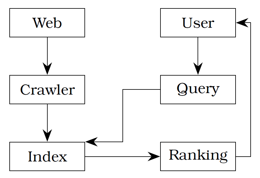
Most big web search engines like Google, Baidu or Bing focus on usefulness and relevance of their results (“Google Ranking” 2012; “Company Overview. About Baidu” n.d.; “Bing Fact Sheet” 2012). Google uses over 200 signals (“Google Ranking” 2012) that influence the ranking of web pages including their original PageRank algorithm (Page et al. 1999; Brin and Page 1998).
Any IR process is constrained by factors like subject, context, time, cost, system and user knowledge (Marchionini and Shneiderman 1988). Such constraints should be taken into consideration in the development of any search tool. A web crawler needs resources to crawl around the web, language barriers may exist, the body of knowledge might not be suitable for all queries, the system might not be able to cater for all types of queries (e.g. single-word vs. multi-word queries), or the user might not be able to understand the user interface, and many more. It is therefore imperative to eliminate certain constraining factors—for example by choosing a specific target audience or filtering the amount of information gathered by a crawler from web pages.
The crawler, sometimes called spider, indexer or bot, is a program that processes and archives information about every available webpage it can find. It does this by looking at given ‘seed’ pages and searching them for hyperlinks. It then follows all of these links and repeats the process over and over. The Googlebot (“Googlebot. Search Console Help” n.d.) and the Bingbot (“Meet Our Crawlers. Webmaster Help and How-to” n.d.) are well-known examples.
An index is a list of keywords (called the dictionary or vocabulary) together with a list called ‘postings list’ that indicates the documents in which the terms occurs. One way to practically implement this is to create a Term-Document Matrix (TDM) as shown in equation 6.1.
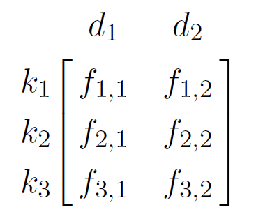
where $f_{i,j}$ is the frequency of term $k_i$ in document $d_j$. To illustrate this with a concrete example, figure 6.2 shows a for a selection of words in a corpus containing three documents1.
Alfred Jarry: Exploits and Opinions of Dr. Faustroll, $′Pataphysician (‘Faustroll’) (1996)
Saint Luke: The Gospel (‘Gospel’) (2005)
Jules Verne: A Journey to the Centre of the Earth (‘Voyage’) (2010)
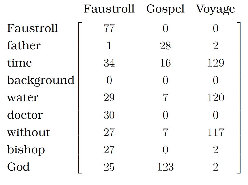
The dictionary is usually pre-processed (see section 6.2) to eliminate punctuation and so-called ‘stop-words’2 (e.g. I, a, and, be, by, for, the, on, etc.) which would be useless in everyday text search engines. For specific domains it even makes sense to build a ‘controlled vocabulary’, where only very specific terms are included (for example the index at the back of a book). This can be seen as a domain specific taxonomy and is very useful for query expansion (explained in the next paragraph).
Relevance feedback is an idea of improving the search results by explicit or implicit methods. Explicit feedback asks users to rate results according to their perceived relevance or collects that kind of information through analysis of mouse clicks, eye tracking, etc. Implicit feedback occurs when external sources are consulted such as thesauri or by analysing the top results provided by a search engine. There are two ways of using this feedback. It can be displayed as a list of suggested search terms to the user and the user decides whether or not to take the advice, or the query is modified internally without the user’s knowledge. This is then called automatic query expansion.
6.1.1 IR Models
There are different models for different needs, for example a multimedia system is going to be different than a text based IR system, and a web based system is going to be different than an offline database system. Even within one such category there could more than one model. Take text based search systems for example. Text can be unstructured or semi-structured. Web pages are typically semi-structured. They contain a title, different sections and paragraphs and so on. An unstructured page would have no such differentiations but only contain simple text. Classic example models are set-theoretic, algebraic and probabilistic. The PageRank algorithm by Google is a link-based retrieval model (Page et al. 1999).
The notation for IR models is a quadruple $[D,Q,F,R(q_i,d_j)]$ (adapted from Baeza-Yates and Ribeiro-Neto 2011) where,
| $D$ | = | the set of documents |
|---|---|---|
| $Q$ | = | the set of queries |
| $F$ | = | the framework e.g. sets, Boolean relations, vectors, linear algebra… |
| $R(q_i, d_j)$ | = | the ranking function, with $q_i ∈ Q$ and $d_j ∈ D$ |
| $t$ | = | the number of index terms in a document collection |
| $V$ | = | the set of all distinct index terms $\{k_1, …, k_t\}$ in a document collection (vocabulary) |
This means, given a query $q$ and a set of documents $D$, we need to produce a ranking score $R(q,d_j)$ for each document $d_j$ in $D$.
The Boolean Model
One such ranking score is the Boolean model. The similarity of document $d_j$ to query $q$ is defined as follows (Baeza-Yates and Ribeiro-Neto 2011)
where $c(x)$ is a ‘conjunctive component’ of $x$. A conjunctive component is one part of a declaration in Disjunctive Normal Form (DNF). It describes which terms occur in a document and which ones do not. For example, for vocabulary $V = \{k_0,k_1,k_2\}$, if all terms occur in document $d_j$ then the conjunctive component would be $(1, 1, 1)$, or $(0, 1, 0)$ if only term $k_1$ appears in $d_j$. Let’s make this clearer with a practical example. Figure 6.3 (a shorter version of figure 6.2) shows a vocabulary of 4 terms over 3 documents.
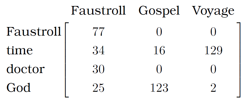
So, we have a vocabulary $V$ of {Faustroll, time, doctor and God} and three documents $d_0=$ Faustroll, $d_1=$ Gospel and $d_2=$ Voyage. The conjunctive component for $d_0$ is $(1, 1, 1, 1)$. This is because each term in $V$ occurs at least once. $c(d_1)$ and $c(d_2)$ are both $(0, 1, 0, 1)$ since the terms ‘Faustroll’ and ‘doctor’ do not occur in either of them.
Assume we have a query $q=$ doctor $∧$ (Faustroll $∨$ $¬$ God). Translating this query into DNF will result in the following expression:
q_{DNF} = (1, 0, 1, 1)∨(1, 1, 1, 1)∨(1, 0, 1, 0)∨(1, 1, 1, 0)∨(0, 0, 1, 0)∨(0, 1, 1, 0)where each component $(x_0, x_1, x_2, x_3)$ is the same as $(x_0 ∧ x_1 ∧ x_2 ∧ x_3)$.
One of the conjunctive components in $q_{DNF}$ must match a document conjunctive component in order to return a positive result. In this case $c(d_0)$ matches the second component in $q_{DNF}$ and therefore the Faustroll document matches the query $q$ but the other two documents do not.
The Boolean model gives ‘Boolean’ results. This means something is either true or false. Sometimes things are not quite black and white though and we need to weigh the importance of words somehow.
TF-IDF
One simple method of assigning a weight to terms is the so-called Term Frequency-Inverse Document Frequency or TF-IDF for short. Given a TF of $tf_{i, j}$ and a IDF of $idf_i$ it is defined as $tf_{i, j} × idf_i$ (Baeza-Yates and Ribeiro-Neto 2011).
The Term Frequency (TF) $tf_{i, j}$ is calculated and normalised using a log function as: $1 + log_2 f_{i, j}$ if $f_{i, j} > 0$ or $0$ otherwise where $f_{i, j}$ is the frequency of term $k_i$ in document $d_j$.
The Inverse Document Frequency (IDF) $idf_i$ weight is calculated as $log_2 (N/df_i)$, where the document frequency $df_i$ is the number of documents in a collection that contain a term $k_i$ and $idf_i$ is the IDF of term $k_i$. The Inverse Document Frequency (IDF) more often a term occurs in different documents the lower the IDF. $N$ is the total number of documents.
where $tfidf_{i, j}$ is the weight associated with $(k_i, d_j)$. Using this formula ensures that rare terms have a higher weight and more so if they occur a lot in one document. Table 6.1 shows the following details.
| $k_0 - k_8$ | = | [Faustroll, father, time, background, water, doctor, without, bishop, God] |
|---|---|---|
| $d_0 - d_2$ | = | [Faustroll, Gospel, Voyage] (see figure 6.2) |
| $f_{i,j}$ | = | the frequence (count) of term $k_i$ in document $d_j$ |
| $tf_{i,j}$ | = | the Term Frequency weight |
| $idf_i$ | = | the Inverse Document Frequency weight |
| $tfidf_{i,j}$ | = | the TF-IDF weight |
What stands out in table 6.1 is that the $tfidf_{i, j}$ function returns quite often. This is partially due to the $idf_i$ algorithm returning when a term appears in all documents in the corpus. In the given example this is the case a lot but in a real-world example it might not occur as much.
The Vector Model
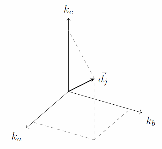
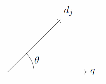
The vector model allows more flexible scoring since it basically computes the ‘degree’ of similarity between a document and a query (Baeza-Yates and Ribeiro-Neto 2011). Each document $d_j$ in the corpus is represented by a document vector $\vec{d_j}$ in $t$-dimensional space, where $t$ is the total number of terms in the vocabulary. Figure 6.4 gives an example of vector $\vec{d_j}$ for document $d_j$ in 3-dimensional space. That is, the vocabulary of this system consists of three terms $k_a$, $k_b$ and $k_c$. A similar vector $\vec{q}$ can be constructed for query $q$. Figure 6.5 then shows the similarity between the document and the query vector as the cosine of $θ$.
$\vec{d_j}$ is defined as $(w_{1, j}, w_{2, j}, …, w_{t, j})$ and similarly $\vec{q}$ is defined as $(w_{1, q}, w_{2, q}, …, w_{t, q})$, where $w_{i, j}$ and $w_{i, q}$ correspond to the TF-IDF weights per term of the relevant document or query respectively. $t$ is the total number of terms in the vocabulary. The similarity between a document $d_j$ and a query $q$ is defined in equation 6.4.
Let’s consider an example similar to the one used for the section. We have a corpus of three documents ($d_0$ = Faustroll, $d_1$ = Gospel, and $d_2$ = Voyage) and nine terms in the vocabulary ($[k_0, …, k_8]$ = (Faustroll, father, time, background, water, doctor, without, bishop, God)). The document vectors and their corresponding length is given below (with the relevant TF-IDF weights taken from table 6.1).
| $\vec{d_0}$ | = | (11.49,0,0,0,0,9.34,0,3.34,0) |
|---|---|---|
| $|\vec{d_0}|$ | = | 15.18 |
| $\vec{d_1}$ | = | (0,0,0,0,0,0,0,0,0) |
| $|\vec{d_1}|$ | = | 0 |
| $\vec{d_2}$ | = | (0,0,0,0,0,0,0,1.16,0) |
| $|\vec{d_2}|$ | = | 1.16 |
For this example we will use two queries: $q_0$ (doctor, Faustroll) and $q_1$ (without, bishop). We then compute the similarity score for between each of the documents compared to the two queries by applying equation 6.4. For the query $q_0$ the result clearly points to the first document, i.e. the Faustroll text. For query $q_1$ the score produces two results, with Verne’s ‘Voyage’ scoring highest.
| $q_0$ | = | (doctor, Faustroll) |
|---|---|---|
| $\vec{q_0}$ | = | (1.58,0,0,0,0,1.58,0,0,0) |
| $|\vec{q_0}|$ | = | 2.24 |
| $sim(d_0,q_0)$ | = | 0.97 |
| $sim(d_1,q_0)$ | = | 0 |
| $sim(d_2,q_0)$ | = | 0 |
| $q_1$ | = | (without, bishop) |
|---|---|---|
| $\vec{q_1}$ | = | (0,0,0,0,0,0,0,0.58,0) |
| $|\vec{q_1}|$ | = | 0.58 |
| $sim(d_0,q_1)$ | = | 0.22 |
| $sim(d_1,q_1)$ | = | 0 |
| $sim(d_2,q_1)$ | = | 1 |

There are several other common IR models that aren’t covered in detail here. These include the probabilistic, set-based, extended Boolean and fuzzy set (Miyamoto 1990a; Miyamoto 1990b; Srinivasan 2001; Widyantoro and Yen 2001; Miyamoto and Nakayama 1986) models or latent semantic indexing (Deerwester et al. 1990), neural network models and others (Macdonald 2009; Schütze 1998; Schütze and Pedersen 1995).
6.1.2 Searching vs. Browsing
What is actually meant by the word ‘searching’? Usually it implies that there is something to be found, an Information Need (IN); although that doesn’t necessarily mean that the searcher knows what he or she is looking for or how to conduct the search and satisfy that need.
From the user’s point of view the search process can be broken down into four activities (Sutcliffe and Ennis 1998) reminiscent of classic problem solving techniques (mentioned briefly in chapter 5.1.1) (Pólya 1957):
- Problem identification
Information Need (IN),
- Need articulation
IN in natural language terms,
- Query formulation
translate IN into query terms, and
- Results evaluation
compare against IN.
This model poses problems in situations where an IN cannot easily be articulated or in fact is not existent and the user is not looking for anything specific. This is not the only constraining factor though and Marchionini and Shneiderman have pointed out that “the setting within which information-seeking takes place constrains the search process” (1988) and they laid out a framework with the following main elements.
Setting (the context of the search and external factors such as time, cost)
Task domain (the body of knowledge, the subject)
Search system (the database or web search engine)
User (the user’s experience)
Outcomes (the assessment of the results/answers)
Searching can be thought of in two ways, ‘information lookup’ (searching) and ‘exploratory search’ (browsing) (Vries 1993; Marchionini 2006). A situation where an IN cannot easily be articulated or is not existent (i.e. the user is not looking for anything specific) can be considered a typical case of exploratory search. The former can be understood as a type of simple question answering while the latter is a more general and broad knowledge acquisition process without a clear goal.
Current web search engines are tailored for information lookup. They do really well in answering simple factoid questions relating to numbers, dates or names (e.g. fact retrieval, navigation, transactions, verification) but not so well in providing answers to questions that are semantically vague or require a certain extend of interpretation or prediction (e.g. analysis, evaluation, forecasting, transformation).
With exploratory search, the user’s success in finding the right information depends a lot more on constraining factors and can sometimes benefit from a combination of information lookup and exploratory search (Marchionini 2006).
Much of the search time in learning search tasks is devoted to examining and comparing results and reformulating queries to discover the boundaries of meaning for key concepts. Learning search tasks are best suited to combinations of browsing and analytical strategies, with lookup searches embedded to get one into the correct neighbourhood for exploratory browsing.
(Marchionini 2006)
De Vries called this form of browsing an “enlargement of the problem space”, where the problem space refers to the resources that possibly contain the answers/solutions to the IN (1993). This is a somewhat similar idea to that of Boden’s conceptual spaces which she called the “territory of structural possibilities” and exploration of that space “exploratory creativity” (Boden 2003) (see section 5.1.6).
6.1.3 Ranking
Ranking signals, such as the weights produced by the TF-IDF algorithm in section 6.6.1.2, contribute to the improvement of the ranking process. These can be content signals or structural signals. Content signals are referring to anything that is concerned with the text and content of a page. This could be simple word counts or the format of text such as headings and font weights. The structural signals are more concerned about the linked structure of pages. They look at incoming and outgoing links on pages. There are also web usage signals that can contribute to ranking algorithms such as the click-stream. This also includes things like the Facebook ‘like’ button or the Google+ ‘+1’ button which could be seen as direct user relevance feedback as well.
Ranking algorithms are the essence of any web search engine and as such guarded with much secrecy. They decide which pages are listed highest in search results and if their ranking criteria were known publically, the potential for abuse (such as ‘Google bombing’ (Nicole 2010) for instance) would be much higher and search results would be less trustworthy. Despite the secrecy there are some algorithms like Google’s PageRank algorithm that have been described and published in academic papers.
Algorithms
PageRank was developed by Larry Page and Sergey Brin as part of their Google search engine (1998; 1999). PageRank is a link analysis algorithm, meaning it looks at the incoming and outgoing links on pages. It assigns a numerical weight to each document, where each link counts as a vote of support in a sense. PageRank is executed at indexing time, so the ranks are stored with each page directly in the index. Brin and Page define the PageRank algorithm as follows (1998).
| $A$ | = | the page we want to rank and is pointed to by pages $T_1$ to $T_n$ |
|---|---|---|
| $n$ | = | the total number of pages on the Web graph |
| $C(A)$ | = | the number of outgoing links of page $A$ |
| $d$ | = | a ‘damping’ parameter set by the system (typically 0.85) needed to deal with dead ends in the graph |
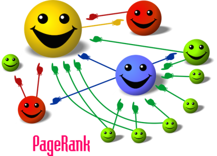
Figure 6.6 which shows how the PageRank algorithm works. Each smiley represents a webpage. The colours are of no consequence. The smile-intensity indicates a higher rank or score. The pointy hands are hyperlinks. The yellow smiley is the happiest since it has the most incoming links from different sources with only one outgoing link. The blue one is slightly smaller and slightly less smiley even though it has the same number of incoming links as the yellow one because it has more outgoing links. The little green faces barely smile since they have no incoming links at all.
The HITS algorithm also works on the links between pages (Kleinberg 1999; Kleinberg et al. 1999). HITS stands for ‘Hyperlink Induced Topic Search’ and its basic features are the use of so called hubs and authority pages. It is executed at query time. Pages that have many incoming links are called ‘authorities’ and page with many outgoing links are called ‘hubs’. Equation 6.6 shows the algorithm (Baeza-Yates and Ribeiro-Neto 2011), where $S$ is the set of pages, $H(p)$ is the hub value for page $p$, and $A(p)$ is the authority value for page $p$.
Hilltop is a similar algorithm with the difference that it operates on a specific set of expert pages as a starting point. It was defined by Bharat and Mihaila (2000). The expert pages they refer to should have many outgoing links to non-affiliated pages on a specific topic. This set of expert pages needs to be pre-processed at the indexing stage. The authority pages they define must be linked to by one of their expert pages. The main difference to the HITS algorithm then is that their ‘hub’ pages are predefined.
Another algorithm is the so called Fish search algorithm (De Bra and Post 1994a; De Bra and Post 1994b; De Bra et al. 1994). The basic concept here is that the search starts with the search query and a seed Uniform Resource Locator (URL) as a starting point. A list of pages is then built dynamically in order of relevance following from link to link. Each node in this directed graph is given a priority depending on whether it is judged to be relevant or not. URLs with higher priority are inserted at the front of the list while others are inserted at the back. Special here is that the ‘ranking’ is done dynamically at query time.
There are various algorithms that follow this approach. For example the shark search algorithm (Hersovici et al. 1998). It improves the process of judging whether or not a given link is relevant or not. It uses a simple vector model with a fuzzy sort of relevance feedback. Another example is the improved fish search algorithm (Luo, Chen, and Guo 2005) where an extra parameter allows more control over the search range and time. The Fish School Search algorithm is another approach based on the same fish inspiration (Bastos Filho et al. 2008). It uses principles from genetic algorithms and particle swarm optimization. Another genetic approach is Webnaut (Nick and Themis 2001).
Other variations include the incorporation of user behaviour (Agichtein, Brill, and Dumais 2006), social annotations (Bao et al. 2007), trust (Gyongyi, Garcia-Molina, and Pedersen 2004), query modifications (Glover et al. 2001), topic sensitive PageRank (Haveliwala 2003), folksonomies (Hotho et al. 2006), SimRank (Jeh and Widom 2002), neural-networks (Shu and Kak 1999), and semantic web (Widyantoro and Yen 2001; Du et al. 2007; Ding et al. 2004; Kamps, Kaptein, and Koolen 2010; Taye 2009).
6.1.4 Challenges
Other issues that arise when trying to search the WWW were identified by Baeza-Yates and Ribeiro-Neto as follows (2011).
Data is distributed. Data is located on different computers all over the world and network traffic is not always reliable.
Data is volatile. Data is deleted, changed or lost all the time so data is often out-of-date and links broken.
The amount of data is massive and grows rapidly. Scaling of the search engine is an issue here.
Data is often unstructured. There is no consistency of data structures.
Data is of poor quality. There is no editor or censor on the Web. A lot of data is redundant too.
Data is not heterogeneous. Different data types (text, images, sound, video) and different languages exist.
Since a single query for a popular word can results in millions of retrieved documents from the index, search engine usually adopt a lazy strategy, meaning that they only actually retrieve the first few pages of results and only compute the rest when needed (Baeza-Yates and Ribeiro-Neto 2011). To handle the vast amounts of space needed to store the index, big search engines use a massive parallel and cluster-based architecture (Baeza-Yates and Ribeiro-Neto 2011). Google for example uses over commodity-class PCs that are distributed over several data centres around the world (Dean, Barroso, and Hoelzle 2003).
6.2 Natural Language Processing
Natural Language Processing (NLP) is a discipline within computer science which is also known as follows (Jurafsky and Martin 2009).
Speech and language processing
Human language technology
Computational linguistics
Speech recognition and synthesis
Goals of NLP are to get computers to perform useful tasks involving human language such as enabling human-machine communication, improving human-human communication, and text and speech processing.Applications are for example machine translation, automatic speech recognition, natural language understanding, word sense disambiguation, spelling correction, and grammar checking.
There are many tools and libraries available for NLP, including the Natural Language Toolkit (NLTK) Python library (Bird, Klein, and Loper 2009; “Natural Language Toolkit. NLTK 3.0 Documentation” n.d.) and WordNet (“What Is Wordnet? WordNet: A Lexical Database for English” n.d.) (both of which were used for pata.physics.wtf).
6.2.1 Words
A ‘lemma’ is a set of lexical forms that have the same stem (e.g. go). A ‘word-form’ is the full inflected or derived form of the word (e.g. goes). A ‘word type’ is a distinct word in a corpus (repetitions are not counted but case sensitive). A ‘word token’ is any word (repetitions are counted repeatedly). Manning et al. list the following activities related to the word processing of text (2009).
- Tokenisation
discarding white spaces and punctuation and making every term a token
- Normalisation
making sets of words with same meanings, e.g. car and automobile
- Case-folding
converting everything to lower case
- Stemming
removing word endings, e.g. connection, connecting, connected → connect
- Lemmatisation
returning dictionary form of a word, e.g. went → go
WordNet
WordNet is a large lexical database for English, containing word form and sense pairs, useful for computational linguistics and NLP (Miller 1995). A synset is a set of synonyms to represent a specific word sense. It is the basic building block of WordNet’s hierarchical structure of lexical relationships.
Nouns, verbs, adjectives and adverbs are grouped into sets of cognitive synonyms (synsets), each expressing a distinct concept. Synsets are interlinked by means of conceptual-semantic and lexical relations.
(WordNet n.d.)
- Synonymy
(same-name) a symmetric relation between word forms
- Antonymy
(opposing-name) a symmetric relation between word forms
- Hyponymy
(sub-name) a transitive relation between synsets
- Hypernymy
(super-name) inverse of hyponymy
- Meronymy
(part-name) complex semantic relation
- Holonymy
(whole-name) inverse of meronymy
- Troponymy
(manner-name) is for verbs what hyponymy is for nouns
Other relations not used by WordNet are homonymy (same spelling but different sound and meaning) and heteronymy (same sound but different spelling), homography (same sound and spelling) and heterography (different sound and spelling).
Appendix C shows an example result produced by WordNet rendered for a web browser.
Regular Expressions
Regular expressions (often shortened to the term ‘regex’) are used to search a corpus of texts for the occurrence of a specific string pattern3.
Table 6.2 shows the most common commands needed to build a regular expression. For example, to find an email address in a piece of text the following regex can be used:
([a-zA-Z0-9_\-\.]+)@([a-zA-Z0-9_\-\.]+)\.([a-zA-Z]{2,5})Most modern text editors support a form of search using regex and it is often used in NLP.
Damerau-Levensthein
The Damerau–Levenshtein distance between two strings $a$ and $b$ is given by $d_{a, b}(|a|,|b|)$ (see equation 6.2) (“Damerau-Levenshtein Distance” n.d.; Damerau 1964; Levenshtein 1966). The distance indicates the number of operations (insertion, deletion, substitution or transposition) it takes to change one string to the other. For example, the words ‘clear’ and ‘clean’ would have a distance of 1, as it takes on substitution of the letter ‘r’ to ‘n’ to change the word. A typical application would be spelling correction.
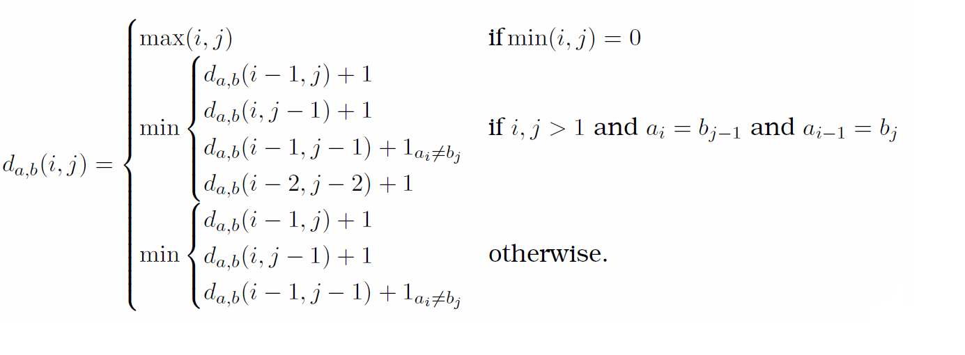
$1_(a_i ≠ b_j)$ is equal to $0$ when $a_i = b_j$ and equal to $1$ otherwise.
$d_{a, b}(i − 1, j)+1$ corresponds to a deletion (from a to b)
$d_{a, b}(i, j − 1)+1$ corresponds to an insertion (from a to b)
$d_{a, b}(i − 1, j − 1)+1_(a_i ≠ b_j)$ corresponds to a match or mismatch, depending on whether the respective symbols are the same
$d_{a, b}(i − 2, j − 2)+1$ corresponds to a transposition between two successive symbols
6.2.2 Sequences
N-Grams
We can do word prediction with probabilistic models called $N$-Grams. They predict the probability of the next word from the previous $N − 1$ words (Jurafsky and Martin 2009). A 2-gram is usually called a ‘bigram’ and a 3-gram a ‘trigram’.
A basic way to compute the probability of an N-gram is using a Maximum Likelihood Estimation (MLE) shown in equation 6.8 (Jurafsky and Martin 2009) of a word $w_n$ given some history $w_{n − N + 1}^{n − 1}$ (i.e. the previous words in the sentence for example).
For instance, if we want to check which of two words “shining” and “cold” has a higher probability of being the next word given a history of “the sun is”, we would need to compute $P$(shining|the sun is) and $P$(cold|the sun is) and compare the results. To do this we would have to divide the number of times the sentence “the sun is shining” occurred in a training corpus by the number of times “the sun is” occurred and the same for the word “cold”.
Counts ($C$) are normalised between 0 and 1. These probabilities are usually generated using a training corpus. These training sets are bound to have incomplete data and certain N-grams might be missed (which will result in a probability of 0). Smoothing techniques help combat this problem.
One example is the so-called ‘Laplace’ or ‘add-one smoothing’, which basically just adds 1 to each count. See equation 6.9 (Jurafsky and Martin 2009). $V$ is the number of terms in the vocabulary.
Another example of smoothing is the so-called ‘Good Turing discounting’. It uses “the count of things you’ve seen once to help estimate the count of things you’ve never seen” (Jurafsky and Martin 2009, their emphasis).
To calculate the probability of a sequence of $n$ words ($P(w_1, w_2, …, w_n)$ or $P(w_{1}^n)$ for short) we can use the chain rule of probability as shown in equation 6.10 (Jurafsky and Martin 2009).
Instead of using the complete history of previous words when calculating the probability of the next term, usually only the immediate predecessor is used. This assumption that the probability of a word depends only on the previous word (or $n$ words) is the called a Markov assumption (see equation 6.11 (Jurafsky and Martin 2009)).
Part-of-Speech Tagging
Parts-of-Speech (POS) are lexical tags for describing the different elements of a sentence. The eight most well-known POS are as follows.
- Noun
an abstract or concrete entity
- Pronoun
a substitute for a noun or noun phrase
- Adjective
a qualifier of a noun
- Verb
an action, occurrence, or state of being
- Adverb
a qualifier of an adjective, verb, or other adverb
- Preposition
an establisher of relation and context
- Conjunction
a syntactic connector
- Interjection
an emotional greeting or exclamation
More specialised sets of tags exist such as the Penn Treebank tagset (Marcus, Santorini, and Marcinkiewicz 1993) consisting of 48 different tags, including $CC$ for coordinating conjunction, $CD$ for cardinal number, $NN$ for noun singular, $NNS$ for noun plural, $NNP$ for proper noun singular, $VB$ for verb base form, $VBG$ for verb gerund, $DT$ for determiner, $JJ$ for adjectives, etc. A full table of these 48 tags can be found in appendix [s:penntreebank].
The process of adding tags to the words of a text is called ‘POS tagging’ or just ‘tagging’. Below, you can see an example tagged sentence4.
In/IN this/DT year/NN Eighteen/CD Hundred/CD and/CC Ninety-eight/CD,/, the/DT Eighth/CD day/NN of/IN February/NNP,/, Pursuant/JJ to/IN article/NN 819/CD of/IN the/DT Code/NN of/IN Civil/NNP Procedure/NNP and/CC at/IN the/DT request/NN of/IN M./NN and/CC Mme./NN Bonhomme/NNP (/(Jacques/NNP)/),/, proprietors/NNS of/IN a/DT house/NN situate/JJ at/IN Paris/NNP,/, 100/CD bis/NN,/, rue/NN Richer/NNP,/, the/DT aforementioned/JJ having/VBG address/NN for/IN service/NN at/IN my/PRP residence/NN and/CC further/JJ at/IN the/DT Town/NNP Hall/NNP of/IN Q/NNP borough/NN ./.Maximum Entropy
Hidden Markov or maximum entropy models can be used for sequence classification, e.g. part-of-speech tagging.
The task of classification is to take a single observation, extract some useful features describing the observation, and then, based on these features, to classify the observation into one of a set of discrete classes.
(Jurafsky and Martin 2009)
A classifier like the maximum entropy model will usually produce a probability of an observation belonging to a specific class. Equation 6.12 shows how to calculate the probability of an obersvation (i.e. word) $x$ being of class $c$ as $p(c|x)$ (Jurafsky and Martin 2009).
| $f_i(c,x)$ | = | the feature (e.g. “this word ends in -ing” or “the previous word was the”) |
|---|---|---|
| $w_i$ | = | the weight of the feature $f_i$ |
Grammars
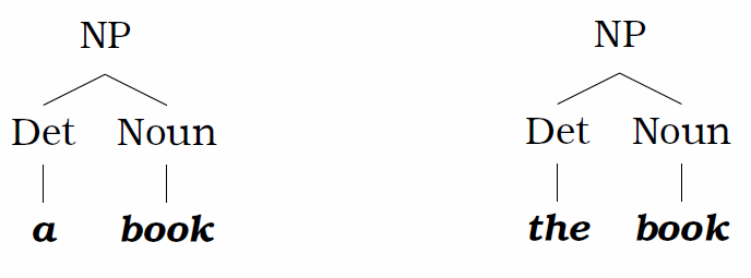
A language is modelled using a grammar, specifically a ‘Context-Free-Grammar’. Such a grammar normally consists or rules and a lexicon. For example a rule could be ‘NP $→$ Det Noun’, where NP stands for noun phrase, Det for determiner and Noun for a noun. The corresponding lexicon would then include facts like Det $→$ a, Det $→$ the, Noun $→$ book. This grammar would let us form two noun phrases ‘the book’ and ‘a book’ only. Its two parse trees would then look like figure 6.7:
Parsing is the process of analysing a sentence and assigning a structure to it. Given a grammar, a parsing algorithm should produce a parse tree for a given sentence. The parse tree for the first sentence from Faustroll is shown below, in horizontal format for convenience.
(ROOT
  (S
    (PP (IN In)
      (NP (DT this) (NN year) (NNPS Eighteen) (NNP Hundred)
        (CC and)
        (NNP Ninety-eight)))
    (, ,)
    (NP
      (NP (DT the) (JJ Eighth) (NN day))
      (PP (IN of)
        (NP (NNP February) (, ,) (NNP Pursuant)))
      (PP
        (PP (TO to)
          (NP
            (NP (NN article) (CD 819))
            (PP (IN of)
              (NP
                (NP (DT the) (NNP Code))
                (PP (IN of)
                  (NP (NNP Civil) (NNP Procedure)))))))
        (CC and)
        (PP (IN at)
          (NP
            (NP (DT the) (NN request))
            (PP (IN of)
              (NP (NNP M.)
                (CC and)
                (NNP Mme) (NNP Bonhomme))))))
      (PRN (-LRB- -LRB-)
        (NP (NNP Jacques))
        (-RRB- -RRB-))
      (, ,)
      (NP
        (NP (NNS proprietors))
        (PP (IN of)
          (NP
            (NP (DT a) (NN house) (NN situate))
            (PP (IN at)
              (NP (NNP Paris))))))
      (, ,)
      (NP (CD 100) (NN bis))
      (, ,))
    (VP (VBP rue)
      (NP
        (NP (NNP Richer))
        (, ,)
        (NP (DT the) (JJ aforementioned)
          (UCP
            (S
              (VP (VBG having)
                (NP
                  (NP (NN address))
                  (PP (IN for)
                    (NP (NN service))))
                (PP (IN at)
                  (NP (PRP$ my) (NN residence)))))
            (CC and)
            (PP
              (ADVP (RBR further))
              (IN at)
              (NP
                (NP (DT the) (NNP Town) (NNP Hall))
                (PP (IN of)
                  (NP (NNP Q))))))
          (NN borough))))
    (. .)))
This particular tree was generated using the Stanford Parser (“The Stanford Parser: A Statistical Parser. the Stanford Natural Language Processing Group” 2016).
Named Entity Recognition
A named entity can be anything that can be referred to by a proper name, such as person, place or organisation names and times and amounts and these entities can be appropriately tagged.
Example (first sentence in Faustroll):
In this [year Eighteen Hundred and Ninety-eight, the Eighth day of February]TIME, Pursuant to article [819]NUMBER of the [Code of Civil Procedure]DOCUMENT and at the request of [M. and Mme. Bonhomme (Jacques)]PERSON, proprietors of a house situate at [Paris, 100 bis, rue Richer]LOCATION, the aforementioned having address for service at my residence and further at the [Town Hall]FACILITY of [Q borough]LOCATION.So-called ‘gazetteers’ (lists of place or person names for example) can help with the detection of these named entities.